Systems Modelling from Scratch (Part 2)
In this blog post we prepare a systems model from scratch — modelling a transition to net-zero steel production for a hypothetical steel plant in Japan. This is the second part of a two-part series introducing the concept of systems modelling and why it is such a power tool for charting a robust pathway to net-zero. Part 1, where we introduce the key concepts of systems modelling, is here.
By Lucas Kruitwagen & Abhishek Shivakumar (with contributions from Ashank Sinha and Badr M’Barek)
There are many possible ‘routes’ to net-zero steel production. Steel production involves the conversion of metallurgical coal, iron ore, energy, and potentially recycled scrap into liquid crude steel. There are many intermediary technologies that can reduce or displace input energy needs and reduce supply chain transport emissions. Several different energy carriers can be used; including electricity, coal, and natural gas. Any one of these intermediary commodities can be shipped between supply, production, and demand geographies. For further reading on the decarbonisation of steel, the EU’s Green Steel for Europe is a good place to start.
For this tutorial, we focus on two routes for primary steel production: the traditional blast furnace + blast oxygen furnace (BF/BOF) route; and the emerging direct reduced iron + electric arc furnace (DRI-EAF) route . The DRI-EAF route offers a potential pathway to decarbonisation whereby hydrogen can displace coal/natural gas in the production of sponge iron and renewable electricity can power the electric arc furnace.
Systems modelling can be used to propose optimal investments of energy and conversion technologies, as well as the volumes of energy and materials that should optimally flow between different conversion technologies and different regions.


The two production routes are illustrated here. These pathways naturally form a directed graph, comprised of nodes for technology plants and commodities.
Let’s explore decarbonisation pathways for a simple steel portfolio in Japan. With a strong automotive industry, Japan is a major steel producer, producing 89mn tonnes in 2022[1]. It is also the second largest exporter of steel in the world, exporting 32mn tonnes in 2022[2]. It imports the required primary materials for production. Since the Fukushima disaster in 2011, Japan’s electricity grid has been dominated by coal and gas generation[3].
Australia and South Africa are both major exporters of iron ore and coal. They also have significant endowments of renewable energy generating potential. Let’s formulate a three-region model to explore options for investment in primary conversion plants in Australia or South Africa. Let’s also consider that certain commodities can be traded on seaborne markets: oil, coal, coke, ore, and direct reduced iron. Which combination of plants, if any, might be optimally relocated to Australia or South Africa under a net-zero pathway?
We will build up a plant-level mixed-integer linear programme to explore this research question.
- We will model each plant individually in each region.
- We’ll have two decision variables: flows
Fon each edge between commodity and plant nodes; and an investment decisionCapExp, representing whether the plant is to be built or not. - We’ll introduce a number of constraints to respect mass balances and technology parameters
- We’ll optimise for least costs, but set a constraint on total carbon emissions
Let’s begin!
Model Setup
Our system model has a graph structure comprised of nodes, representing our plants, and edges, along which flows can traverse the graph. Supply of each commodity must traverse the graph from the nodes where it is produced to nodes where it is demanded. Edges exist between each node and each plant accepting the commodity as inputs. The capacity of the edges is determined by the investment decision variable of the model — full capacity if the investment decisions is made, (i.e. CapExp=1) and zero otherwise. Total system costs to be minimised are the combination of both opex as a function of flows and capex from capital investment. The graph below is repeated for every commodity and technology, in every region, at every timestep.

Let’s import our Python packages. We’ll use NetworkX to assemble our data in a graph structure. We’ll then turn our graph into a linear programme using PuLP. Finally we’ll import Pydantic’s BaseModel and a few itertools to help us structure our data.
from itertools import chain, product
import json
from pulp import *
import networkx as nx
from pydantic import BaseModel
Systems models being with several sets that define the dimensions of our model. YEARS define the time dimension of our model. To reduce the complexity of our model, we sample every 5 years. COMMODITIES are the various flows of energy and materials that move through our model. We define external, internal, and target commodities, as well as commodities that can be transportable between regions.
YEARS = list(range(2020,2055,5))
EXT_COMMODITIES = ['ORE','COAL','OIL','NATGAS','RENS','SCRAP']  # t_ore, t_coal, t_oil, GJ, GJ, t_scrap
INT_COMMODITIES = ['NATGAS_OR_H2','COKE','HOTMET','DRI','H2','ELEC','HOTMET_OR_SCRAP','HEAT'] # GJ, t_hotmet, t_dri, GJ, GJ, t_hm_or_scrap, GJ
TARGET_COMMODITIES = ['STEEL']
TRANSPORTABLE_COMMODITIES = ['ORE','COAL','COKE','DRI']
COMMODITIES = EXT_COMMODITIES + INT_COMMODITIES + TARGET_COMMODITIES
Next we define the spatial REGIONS of our model. Our model comprises Japan (JP), South Africa (ZA), and Australia (AU). We also define the distances between each region that we can use in our calculations later. Not every commodity is available in each region. We define some variable costs for the available resources in each region, and a unit-tonne freight cost for transferring resources between regions.
REGIONS = {
    'JP':Region(
        id='JP', # Japan
        available_resources=['OIL','NATGAS','SCRAP','RENS'],
        resource_varcost = {
          'OIL':120*7.3, # $/t
          'NATGAS':23, # $/GJ
          'RENS':0, # $/GJ
          'SCRAP':2204*0.24 # $/t
        },
    ),
    'ZA':Region(
        id='ZA', # South Africa
        available_resources=['OIL','NATGAS','RENS', 'COAL','ORE','SCRAP'],
        resource_varcost = {
          'OIL':70*7.3, # $/t
          'NATGAS':40, # $/GJ
          'RENS':0, # $/GJ
          'ORE':100, # $/t
          'COAL':30, #$/t
          'SCRAP':2204*0.24 # $/t
        },
    ),
    'AU':Region(
        id='AU', # Australia
        available_resources=['OIL','NATGAS','RENS','COAL','ORE','SCRAP'],
        resource_varcost = {
          'OIL':70*7.3, # $/t,
          'NATGAS':20, # $/GJ,
          'RENS':0, # $/GJ,
          'ORE':105, # $/t,
          'COAL':40, # $/t,
          'SCRAP':2204*0.24 # $/t
        },
    )
}

DISTANCES = {
    ('JP','AU'):6500, # km
    ('ZA','JP'):14000, # km
    ('AU','ZA'):9000, #km
}

OCEAN_FREIGHT_RATE = 0.01 # $/t/km (China->US $4/kg)

FREIGHT_COSTS = {kk:vv*OCEAN_FREIGHT_RATE for kk,vv in DISTANCES.items()} # $/t
The physics of systems modelling rely on the continuity equations: the balance of energy and materials at each node must be zero, net of any additional supply and demand. For this model, for each year, the demand of steel should be 65 tonnes per annum, otherwise zero.
DEMAND = {
  (region.id,year,commodity):65
  if (commodity=='STEEL' and region.id=='JP')
  else 0
  for region, year, commodity in product(REGIONS.values(), YEARS, COMMODITIES)
}
For convenience we also sum the demand in each year.
DEMAND_SUM_IN_YEAR = {
  year:sum(
    [DEMAND[(region.id, year, commodity)]
    for region, commodity
    in product(REGIONS.values(),COMMODITIES)]
  )
  for year in YEARS
}
We need to be able to constrain system emissions to explore pathway options. Using the system mass balance, all emissions are derived from the input fuels as well as the transport freight. We define some emissions_factors to be used in calculating system emissions.
# emissions factors
emissions_factors = {
    'COAL': 2860, # kg/t_coal,
    'OIL':1800, # kg/t_oil
    'NATGAS': 50, # kg/GJ
    'FREIGHT':0.0063, # kg_co2e/t/km
}
for edge_key, distance in DISTANCES.items():
    emissions_factors[edge_key] = emissions_factors['FREIGHT']*distance # kg_co2e/t
Lastly, we define some limits to the amount of hydrogen that can displace natural gas, and the amount of scrap material that can be recycled as an input to final steel production.
MAX_H2_NG_RATIO = 0.9
MAX_SCRAP_RATIO = 0.3
Adding Plants
Now it’s time to define our potential plants. We begin with some PlantArchetypes: defaults for each of our plant types. We can define plants as generic objects with inputs, outputs, capital expenditure (capex), operational expenditure (opex), and lifespans, and use this template for all our required plant types: [direct_reduced_iron, electric_arc_furnace, coking_plant, blast_furnace, basic_oxygen_furnace, hydrogen_electrolyser, coal_powerstation, natural_gas_powerstation, oil_powerstation, renewable_powerstation, coal_heat_plant, natural_gas_heat_plant, oil_heat_plant]. We also define a Plant class which describes a single plant instance based on an archetype.
class PlantArchetype(BaseModel):
    """ Represents a single potential plant"""
    archetype: str  # plant archetype code
    unit_capex: int  # $
    opex: int  # $/OUTPUT unit
    lifespan: int  # years
    commodity_input_ratio: dict  # INPUT commodity {KEY:ratio}
    commodity_output: str  # OUTPUT commodity
    inp_nodes: Optional[list] = None
    outp_nodes: Optional[list] = None
    capexp_node: Optional[str] = None


class Plant(PlantArchetype):
    """ Represents a single potential plant"""
    id: str  # id
    availability_year: int  # first year
    capacity: float  # OUTPUT {key:value}
    region_id: str
    active_years: Optional[list] = None
We need to populate our PlantArchetypes from data. We can draw on plant defaults from TransitionZero’s Steel Archetype Tracker, reproduced here and copied into a gist for convenience. Plants have one-or-more input commodities which are converted into one unit of commodity_output at a rate described by commodity_input_ratio.
+-------------+------------+------+----------+---------------------------------------------+------------------+
|  archetype  | unit_capex | opex | lifespan |            commodity_input_ratio            | commodity_output |
+-------------+------------+------+----------+---------------------------------------------+------------------+
| coke        |        235 |   17 |       20 | {'COAL': 1.38; 'ELEC': 0.3744}              | COKE             |
| bf          |        159 |    9 |       15 | {'COKE': 0.653; 'ORE': 1.5; 'HEAT': 3.25}   | HOTMET           |
| bof         |        104 |   41 |       15 | {'HOTMET_OR_SCRAP': 1}                      | STEEL            |
| eaf         |        217 |   68 |       20 | {'ELEC': 1.512; 'DRI': 1}                   | STEEL            |
| dri         |        258 |    8 |       20 | {'NATGAS_OR_H2': 9.62; 'ORE': 1.6}          | DRI              |
| h2          |         78 |    0 |       15 | {'ELEC': 1.710}                             | H2               |
| coal_ps     |         19 |    0 |       40 | {'COAL': 0.1041}                            | ELEC             |
| natgas_ps   |         25 |    0 |       40 | {'NATGAS': 1.667}                           | ELEC             |
| oil_ps      |         31 |    0 |       40 | {'OIL': 0.0649}                             | ELEC             |
| ren_ps      |         79 |    0 |       25 | {'RENS': 1}                                 | ELEC             |
| coal_heat   |          7 |    0 |       40 | {'COAL': 0.04167}                           | HEAT             |
| natgas_heat |         15 |    0 |       40 | {'NATGAS': 1}                               | HEAT             |
| oil_heat    |         11 |    0 |       40 | {'OIL': 0.0227}                             | HEAT             |
+-------------+------------+------+----------+---------------------------------------------+------------------+
archetype_df = pd.read_csv('https://gist.githubusercontent.com/Lkruitwagen/59bca62d375aa510103844051e970898/raw/59c7e37314d43a836a376ede43062f40085e18f7/archetypes.csv')
# map json.loads to load dict data
archetype_df['commodity_input_ratio'] = archetype_df['commodity_input_ratio'].apply(json.loads)
archetype_plants = {
row['archetype']:PlantArchetype(**row.to_dict()) #
for idx, row in archetype_df.iterrows()
}We can then use our archetypes to instantiate all the plants for our model. In every region we define a set of potential plants. We allow plants to be built from a discrete set of plant_potential_capacities. One plant of each capacity is available in each year in each region. We’ll only add a basic differentiation between regions, which is to make renewables in Japan 150% more expensive than in Australia or South Africa.
plant_potential_capacities = {
    'coking':[35,70],    # 35t, 70t
    'bf':[35,70],
    'bof':[35,70],
    'eaf':[35,70],
    'dri':[35,70],
    'h2':[35,350,700],
    'coal_ps':[25,100,250],
    'natgas_ps':[25,100,250],
    'oil_ps':[25,100,250],
    'ren_ps':[25,100,250,1000,2000],
    'coal_heat':[25, 100, 250],
    'natgas_heat':[25,100,250],
    'oil_heat':[25,100,250]
}

all_plants = []
for (plant_key, capacities_list),region in product(plant_potential_capacities.items(), REGIONS.values()):
    for capacity, year in product(capacities_list, YEARS):
        all_plants.append(
            Plant(
                **archetype_plants[plant_key].__dict__,
                id = f"PLANT-{plant_key}-{year}-{capacity}-{region.id}",
                capacity=capacity,
                availability_year=year,
                region_id=region.id,
            )
        )

# make renewables in Japan more expensive
for p in all_plants:
    if p.archetype=='ren_ps' and p.region_id=='JP':
        p.unit_capex *= 1.5
To account for the fact that a set of plants already exists in Japan, we define an initial set of plants that can provide the complete steel supply chain and add these to all plants for the model. To account for the fact that these plants already exist, the unit_capex of these plants is set to 0, the model can build them ‘for free’.
initial_plants_jp = [
    Plant(
        **archetype_plants['coking'].__dict__,
        id='PLANT-coking-ini-jp',
        capacity=70, # 70 t_coke / yr
        availability_year = 2015,
        region_id='JP',
    ),
    Plant(
        **archetype_plants['bf'].__dict__,
        id='PLANT-bf-ini-jp',
        capacity=70, # 70 t_hotmet / yr
        availability_year = 2015,
        region_id='JP',
    ),
    Plant(
        **archetype_plants['bof'].__dict__,
        id='PLANT-bof-ini-jp',
        capacity=70, # 70 t_steel / yr
        availability_year = 2015,
        region_id='JP',
    ),
    Plant(
        **archetype_plants['coal_ps'].__dict__,
        id='PLANT-coal_ps-ini-jp',
        capacity=25, # 25GJ_elec/yr
        availability_year = 2000,
        region_id='JP',
    ),
    Plant(
        **archetype_plants['coal_heat'].__dict__,
        id='PLANT-coal_heat-ini-jp',
        capacity=250, # 250 GJ_heat/yr
        availability_year = 2000,
        region_id='JP',
    )
]

# initial (existing) plants have no capex
for p in initial_plants_jp:
    p.unit_capex = 0.

# add initial plants
all_plants += initial_plants_jp
We now have everything we need to build our network object.
Building the Graph
We can now build our NetworkX directional graph. We begin by initialising our graph and adding ‘buses’ for each commodity in each region, and all our plants.
G = nx.DiGraph()

commodity_region_buses = [
    (
        '-'.join([commodity,region.id,str(year)]),
        {'type':'BUS'}
    )
    for commodity, region, year in product(COMMODITIES,REGIONS.values(), YEARS)
]

G.add_nodes_from(commodity_region_buses)

# add existing plants and new plants
for plant in all_plants:
    plant.active_years = [year for year in YEARS if (year>= plant.availability_year and year<= (plant.availability_year+plant.lifespan))]
    plant_nodes = [(f'{plant.id}-{year}',{'type':'PLANT'}) for year in plant.active_years]
    G.add_nodes_from(plant_nodes)

# catalog all plants by id
plants_dict = {p.id:p for p in all_plants}
Our system needs to have aggregate balance between supply and demand. We need to add some extra nodes for each input and output commodity than can act as global supply sources and demand sinks.
# add supply nodes
global_demand = sum(YEAR_DEMAND.values())

optim_nodes = [
    ('GLOBAL_STEEL_DEMAND',{'demand':global_demand, 'type':'TARGET'})
]

optim_nodes += [
    (f'GLOBAL_{inp}_SUPPLY',{'demand':0})
    for inp in EXT_COMMODITIES
]

G.add_nodes_from(optim_nodes)
We now have all the plants populated in our graph object as nodes. It’s time to connect the plants with edges for material and energy flows. A LARGE_VAL is defined for pseudo-infinite capacity edges. Input and output edges are defined for each respective commodity in each year.
input_edges = [
    (
        f'GLOBAL_{commodity}_SUPPLY',
        '-'.join([commodity,region.id,str(year)]),
        {
            'capacity':LARGE_VAL,
            'cost_var':region.resource_varcost[commodity],
            'cost_fixed':0
        }
    )
    for commodity, region, year in product(EXT_COMMODITIES, REGIONS.values(), YEARS) if commodity in region.available_resources
]

output_edges = [
    (
        '-'.join(['STEEL',region.id,str(year)]),
        'GLOBAL_STEEL_DEMAND',
        {
            'capacity':DEMAND[(region.id, year, commodity)],
            'cost_var':0,
            'cost_fixed':0
        }
    )
    for commodity, region, year in product(TARGET_COMMODITIES, REGIONS.values(), YEARS)
]

G.add_edges_from(output_edges)
G.add_edges_from(input_edges)
The edges between each commodity and each plant are constrained by the production capacity of the plant.
for plant in all_plants:
    input_plant_edges =  [
        (
            '-'.join([commodity,plant.region_id,str(year)]),
            f'{plant.id}-{year}',
            {
                'capacity':plant.capacity*ratio,
                'ratio':ratio,
                'cost_var':0,
                'cost_fixed':0
            }
        )
        for (commodity, ratio),year in product(plant.commodity_input_ratio.items(), plant.active_years)
    ]

    output_plant_edges = [
        (
            f'{plant.id}-{year}',
            '-'.join([plant.commodity_output,plant.region_id,str(year)]),
            {
                'capacity':plant.capacity,
                'cost_var':plant.opex,
                'cost_fixed':0
            }
        )
        for year in plant.active_years
    ]

    G.add_edges_from(input_plant_edges+output_plant_edges)
We also need to add the edges between each pair of regions. These edges are reversible — transportable commodities can flow in either direction. We use our freight tonnage cost from earlier as our variable cost.
## add transport edges
for commodity, year in product(TRANSPORTABLE_COMMODITIES, YEARS):
    forward_edges = [
        (
            '-'.join([commodity, src, str(year)]),
            '-'.join([commodity, dest, str(year)]),
            {
                'capacity':LARGE_VAL,
                'cost_var':val,
                'cost_fixed':0
            }
        )
        for (src, dest), val in FREIGHT_COSTS.items()
    ]

    reverse_edges = [
        (
            '-'.join([commodity, dest, str(year)]),
            '-'.join([commodity, src, str(year)]),
            {
                'capacity':LARGE_VAL,
                'cost_var':val,
                'cost_fixed':0
            }
        )
        for (src, dest), val in FREIGHT_COSTS.items()
    ]

    G.add_edges_from(forward_edges+reverse_edges)
Finally we need some ‘either-or’ edges. These are edges that can carry either of two commodities — the model will choose the cost-optimal combination of the two.
## add 'either or' edges
# 'SCRAP','HOTMET' -> 'HOTMET_OR_SCRAP'
# 'NATGAS',H2' ->'NATGAS_OR_H2'
scrap_or_hotmet_edges = [
    (
        '-'.join([commodity,region.id,str(year)]),
        '-'.join(['HOTMET_OR_SCRAP',region.id,str(year)]),
        {
            'capacity':LARGE_VAL,
            'cost_var':0,
            'cost_fixed':0
        }
    )
    for commodity, region, year in product(['SCRAP','HOTMET'],REGIONS.values(), YEARS)
]

ng_or_h2_edges = [
    (
        '-'.join([commodity,region.id,str(year)]),
        '-'.join(['NATGAS_OR_H2',region.id,str(year)]),
        {
            'capacity':LARGE_VAL,
            'cost_var':0,
            'cost_fixed':0
        }
    )
    for commodity, region, year in product(['NATGAS','H2'],REGIONS.values(), YEARS)
]

G.add_edges_from(scrap_or_hotmet_edges+ng_or_h2_edges)
Building the Model
With our graph fully described, it is now an easier task to build our model. We’ll be using PuLP to define our linear programme, but there are many similar libraries available. PuLP has an easy, expressive approach which makes it friendly for beginners. We start by instantiating a model object.
model = LpProblem("graph_model_mincostflow",LpMinimize)Our model has a name, graph_model_mincostflow , and an objective, LpMinimize. Our objective will be to minimize some function (which we have yet to define.)
Next we’ll add our decision variables; these are the variables we want the model to decide for us. For our problem, like many system modelling problems, there are only two decision variables: a flow variable and an investment variable. Flows are continuous with a lower bound of zero; capital expenditure (CapExp) is constrained to integer values equal to 0 or 1, representing the decision to invest in the plant or not. (This integer constraint is what makes this a mixed-integer linear programme, as opposed to a linear programme only.)
# decision variables; only 2:
F = LpVariable.dicts("Flows",list(G.edges), lowBound=0, cat='continuous')
capexp = LpVariable.dicts("CapExp", list(plants_dict.keys()), 0,1, LpInteger)
Adding constraints to our model using our graph object is now straight-forward. First, at every node, the sum or all flows, supply and demands must equal zero.
# for every node, sum(flows) + demand == 0
for n, params in G.nodes.items():
    # for buses, sum(flows) == 0
    node_type = params.get('type')

    if node_type=='BUS':
        # for buses, sum(flows)==0
        model += sum([F[e_i] for e_i in G.in_edges(n)])-sum([F[e_o] for e_o in G.out_edges(n)]) == 0

    if node_type=='PLANT':
        # for plants, input_flows >= ratio*output_flow
        e_o = list(G.out_edges(n))[0]
        for e_i in G.in_edges(n):
            model+=  F[e_i] >= F[e_o]*G.edges[e_i]['ratio']

    if node_type=='TARGET':
        # for our target nodes, set sum(flows) - demand == 0
        model += sum([F[e_i] for e_i in G.in_edges(n)])-sum([F[e_o] for e_o in G.out_edges(n)]) - params.get('demand',0) == 0
Next, we need to constrain the input and output edge capacities. Input and output edge capacities must be less than the plant capacity time the CapExp variable for that plant.
# for every edge, constrain capacity
for (n_s, n_t), data in G.edges.items():
    if 'PLANT' in n_s:
        p_id = '-'.join(n_s.split('-')[0:-1])
        model += F[(n_s, n_t)] <= data['capacity'] * capexp[p_id]
    elif 'PLANT' in n_t:
        p_id = '-'.join(n_t.split('-')[0:-1])
        model += F[(n_s, n_t)] <= data['capacity'] * capexp[p_id]
    else:
        model += F[(n_s, n_t)] <= data['capacity']
Finally, for the ‘either-or’ nodes, the ratio of the two inputs must be constrained.
# constrain 'either or' edge bundles
for n, params in G.nodes.items():

    node_type = params.get('type')

    if node_type=='BUS' and 'HOTMET_OR_SCRAP' in n:
        # sum(SCRAP) <= max_scrap / (1-max_scrap)*sum(HOTMET)
        model += sum([F[e_i] for e_i in G.in_edges(n) if 'SCRAP' in e_i[0]]) <= (MAX_SCRAP_RATIO/(1-MAX_SCRAP_RATIO)) * sum([F[e_i] for e_i in G.in_edges(n) if 'HOTMET' in e_i[0]])

    if node_type=='BUS' and 'NATGAS_OR_H2' in n:
        # sum(H2) <= max_scrap / (1-max_scrap)*sum(NATGAS)
        model += sum([F[e_i] for e_i in G.in_edges(n) if 'H2' in e_i[0]]) <= (MAX_H2_NG_RATIO/(1-MAX_H2_NG_RATIO)) * sum([F[e_i] for e_i in G.in_edges(n) if 'NATGAS' in e_i[0]])
With all the equations generated, we can now generate the total system costs to minimise. We define costs_flow and costs_capexp as affine equations — linear combinations of other system variables. We then add these two values together into costs_total, the total cost of the system, the variable the model will seek to minimise.
### OPTIM  CRITERIA
costs_flow = [F[(n_s, n_t)] * e_data['cost_var'] for (n_s, n_t), e_data in G.edges.items()]
costs_capexp = [capexp[p_id] * plants_dict[p_id].unit_capex * plants_dict[p_id].capacity for p_id in capexp.keys()]
costs_total = sum(costs_flow) + sum(costs_capexp)
model += costs_total, "Total Cost"
For convenience, we’ll define define some more affine equations — this time for carbon emissions from our three fossil energy carriers as well as inter-regional transport. We can use these equations later.
### other affine equations -> emissions
emissions_oil_yearly = {year:sum([F[e]*emissions_factors['OIL'] for e in G.out_edges('GLOBAL_OIL_SUPPLY') if str(year) in e[1]]) for year in YEARS}
emissions_coal_yearly = {year:sum([F[e]*emissions_factors['COAL'] for e in G.out_edges('GLOBAL_COAL_SUPPLY') if str(year) in e[1]]) for year in YEARS}
emissions_gas_yearly = {year:sum([F[e]*emissions_factors['NATGAS'] for e in G.out_edges('GLOBAL_NATGAS_SUPPLY') if str(year) in e[1]]) for year in YEARS}
transport_emissions_yearly = {
    year:sum(
        [F[('-'.join([commodity, src, str(year)]),'-'.join([commodity, dest, str(year)]))]*emissions_factors[(src,dest)] for commodity, ((src, dest),_) in product(TRANSPORTABLE_COMMODITIES, FREIGHT_COSTS.items())] +
        [F[('-'.join([commodity, dest, str(year)]),'-'.join([commodity, src, str(year)]))]*emissions_factors[(src,dest)] for commodity, ((src, dest),_) in product(TRANSPORTABLE_COMMODITIES, FREIGHT_COSTS.items())]
    )
    for year in YEARS
}

emissions_yearly = {
    year:sum([
        emissions_oil_yearly[year],
        emissions_gas_yearly[year],
        emissions_coal_yearly[year],
        transport_emissions_yearly[year],
    ])
    for year in YEARS
}
We’re finally ready to solve our model. We have several options for which optimiser we user. COIN-OR CBC is a widely used open-source option. Academics may also have options to more powerful options like Gurobi.
model.solve(PULP_CBC_CMD())Analysis
We’re now ready to use our systems model for some analysis. Let’s run four cases, or scenarios:
- We’ll run our first baseline scenario as a benchmark. This scenario will be unconstrained by emissions and will simply minimise system costs
- The second scenario will be a decarbonisation-2050 scenario. In this scenario, scope steel production must reduce emissions to less than 25% by 2050 and must halve by 2035.
- The third scenario will be a decarbonisation-2040 scenario. In this scenario, scope steel production must reduce emissions to less than 25% by 2040 and must halve by 2030.
- In our final scenario, no-import we will constrain our decarbonisation-2040 scenario such that no products other than energy products can be imported to Japan.
To retrieve results from our model, we can easily use the variables and affine equations we defined during model creation. After we solve our model, we can obtain the solved data from these variables. The code for parsing this data and rendering it into some figures is included after the jump below.
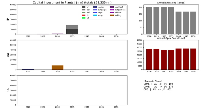
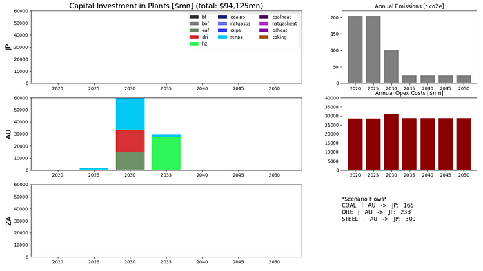
Scenario 1: Baseline
Our first scenario is a baseline scenario. In this scenario, there is no constraint on carbon emissions. In the capital investments, coal power stations, blast furnace, and blast oxygen furnace are built in 2030 and 2035 and provide all steel production capacity through the model period. A coking plant is built in Australia and coke is shipped from Australia to Japan.
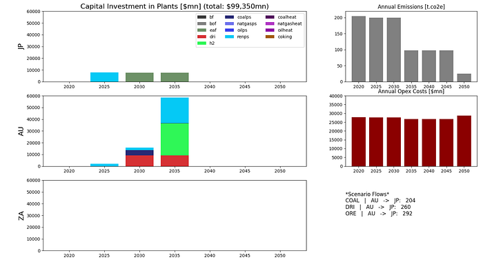
Scenario 2: Decarbonisation 2050
In this second scenario, system emissions must be less than 25 tonnes co2e per year by 2050, and less than 100 tonnes co2e by 2035. This can be done by adding the following constraints to the model prior to the solve:
model += emissions_yearly[2035] <= 100000
model += emissions_yearly[2050] <= 25000
With these constraints, we see significant investment in renewables in Japan and Australia. Electric arc furnaces are built in Japan in the 2030s, and DRI facilities are build in Australia, alongside some coal power generation. DRI is shipped from Australia to Japan. Capital investment is almost triple the baseline scenario.
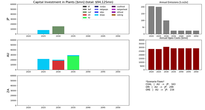
Scenario 3: Decarbonisation 2040
With this third scenario, ambition is increased to significantly decarbonise steel production by 2040. The following constraints are added prior to the model solve:
model += emissions_yearly[2030] <= 100000
model += emissions_yearly[2040] <= 25000
model += emissions_yearly[2045] <= 25000
model += emissions_yearly[2050] <= 25000
In this scenario, only renewable generating capacities are installed. Significant DRI processing facilties are built in Australia, and EAF capacity built in Japan. Renewables capacity is built in Australia prior to 2030, unlike in the later decarbonisation scenario. Total capital investments are about the same as in the later decarbonisation scenario.
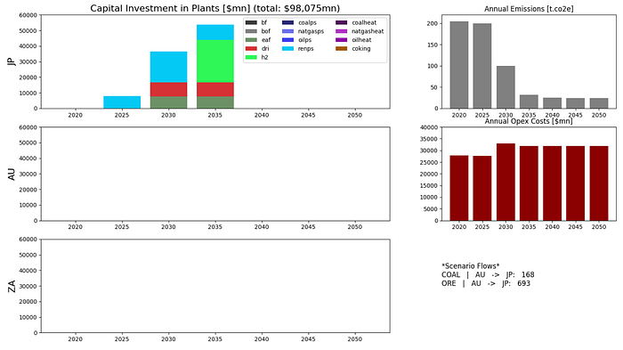
Scenario 4: Decarbonisation 2040 — no transport of coke or DRI
This scenario has the same 2040 decarbonisation target, but does not allow coke or DRI transport:
TRANSPORTABLE_COMMODITIES = ['ORE','COAL']In this scenario, we see significant build-out of renewable generating capacity and electrolysis in Japan only, alongside DRI and EAF capacity. Operating expenditures are significantly higher with this constraint.
Scenario 5 — bonus — allow transport of steel
If the transport of steel is allowed, we see DRI, EAF, electrolysis, and renewable generation capacity move to Australia.
In none of the scenarios analysed did we see any building of capacity in South Africa.
Conclusion
This tutorial demonstrated how systems models can be built from scratch, and how they are powerful tools for analysis — allowing quick iteration between counterfactual views of the future. Designing data structures in graphs allows systems models to be constructed logically and efficiently. It should be clear how the toy model developed here could be iterated and expanded to provide a powerful engine for investment decision-making.
The code used in this tutorial is available in a jupyter notebook here.
Annex: figure generation code from model results
transport_records = []
for key, f in F.items():
    if key[0].split('-')[0] == key[1].split('-')[0]:
        transport_records.append({
            'commod':key[0].split('-')[0],
            'year':key[0].split('-')[-1],
            'src':key[0].split('-')[1],
            'dst':key[1].split('-')[1],
            'val':f.value(),
        })
transport_df = pd.DataFrame(transport_records)
transport_df = transport_df.groupby(['commod','src','dst'])['val'].sum().reset_index()
flow_vals = [{'key':list(c.keys())[0],'value':c.value()} for c in costs_flow if len(c.keys())>0]
flow_val_df = pd.DataFrame(flow_vals)
flow_val_df['year'] = flow_val_df['key'].astype(str).str.split('_').str[-1].str[0:4].astype(int)
key_vals = [{'key':list(c.keys())[0],'value':c.value()} for c in costs_capexp if len(c.keys())>0]
key_df = pd.DataFrame(pd.DataFrame(key_vals)['key'].astype(str).str.split('_').tolist(), columns=['null0','null1','plant','year','capacity','region'])
df = pd.merge(
    pd.DataFrame(key_vals),
    pd.DataFrame(pd.DataFrame(key_vals)['key'].astype(str).str.split('_').tolist(), columns=['null0','null1','plant','year','capacity','region']),
    how='left',
    left_index=True,right_index=True
)
total_capex = df['value'].sum()
plant_types=archetype_plants.keys()
annual_emissions = {year:emissions_yearly[int(year)].value() for year in years}
cmap = dict(zip(
    ['bf', 'bof', 'eaf', 'dri', 'h2', 'coalps', 'natgasps', 'oilps', 'renps', 'coalheat', 'natgasheat', 'oilheat', 'coking'],
    ['#3b3b3b','#808080','#6d9167','#d63134','#2ff757','#282a75','#6d71ed','#3b40ed','#05c9f5','#53115e','#b035c4','#8d07a3','#a35a07']
))
bar_data = {}
for region in ['JP','AU','ZA']:
    bar_data[region] = {}
    for plant_type in archetype_plants.keys():
        bar_data[region][plant_type] = df.loc[(df['region']==region)&(df['plant']==plant_type)].groupby('year')['value'].sum().values
annotated_str = "\n".join([f"{row.commod}   |   {row.src}   ->   {row.dst}:   {row.val:.0f}" for idx, row in transport_df.loc[transport_df['val']>0].iterrows()])
annotated_str = "*Scenario Flows*\n" + annotated_str
fig, ax= plt.subplots(3,2,figsize=(18,10), width_ratios=[2, 1])
years = np.arange(2020,2055,5)
for ii_r, region in enumerate(bar_data.keys()):
    bottom = np.zeros(7)
    for ii_p, plant_type in enumerate(bar_data[region].keys()):
        ax[ii_r][0].bar(years, bar_data[region][plant_type], 4, label=plant_type, bottom=bottom, color=cmap[plant_type])
        bottom += bar_data[region][plant_type]
        ax[ii_r][0].set_ylabel(region, fontsize=16)
        ax[ii_r][0].set_ylim([0,60000])
ax[0][0].legend(ncols=3, loc='upper right')
ax[0][0].set_title(f'Capital Investment in Plants [$mn] (total: \${total_capex:,.0f}mn)', fontsize=16)
ax[0][1].bar(annual_emissions.keys(), np.array(list(annual_emissions.values()))/1000, color='gray', width=4)
ax[0][1].set_ylim([0,220])
ax[1][1].bar(flow_val_df.groupby('year')['value'].sum().index, flow_val_df.groupby('year')['value'].sum().values, color='darkred', width=4)
ax[0][1].set_title('Annual Emissions [t.co2e]')
ax[1][1].set_title('Annual Opex Costs [$mn]')
ax[1][1].set_ylim([0,40000])
ax[2][1].axis('off')
ax[2][1].annotate(annotated_str,(0,0.5), fontsize=12)
[1]: https://www.statista.com/statistics/630041/japan-crude-steel-production/
[2]: https://www.statista.com/statistics/1304737/japan-customs-export-volume-value-iron-steel-products/
[3]: https://ourworldindata.org/energy/country/japan
