Systems Modelling from Scratch (Part 1)
In this tech blog we introduce the concept of Systems Modelling — and why it is such a powerful tool for charting a robust pathway to net-zero. In Part 1, we discuss how a systems model is designed and optimised, and some of the limits to these tools. In Part 2, we prepare a systems model from scratch for a sector-coupled steel supply chain.
By Lucas Kruitwagen & Abhishek Shivakumar
As humanity approaches planetary boundaries in carbon, water, and biodiversity, we face difficult choices about the trade-offs between sustainability, conservation, socialized costs, intergenerational equity, growth, and poverty eradication. Many of our human socio-techno-economic systems (e.g. food production, energy production, the built environment, transportation, etc. and finance and investment there-in) have complex interactions with our biosphere and one-or-more of these planetary boundaries. The future is uncertain due to both stochastic phenomena like the weather, but also social phenomena like policy choices and changing consumer preferences. Decision-makers in both private and public spheres need tools to help them navigate these uncertainties; assessing resilience, testing counterfactuals, and identifying decision-making optima. Quantifying these trade-offs, and what they mean for our collective future, empowers decision makers to navigate the complexities of the 21st century — and ensures that such decisions are accountable to public welfare and open debate.

Systems modelling seeks to identify and characterise the relationships between the diverse elements of these complex systems. They were first used in the energy domain in response to the oil price shocks in 1973 — facilitating preparation in the face of an uncertain future. While these original models focused on the optimal allocation and routing of oil products, they have since expanded to cover the entire energy system. As we reach the limits of our biosphere’s ability to absorb anthropocentric carbon emissions, energy system models are now being applied to task of navigating the uncertainties of delivering a net-zero energy system. The unfolding energy transition requires a fundamental transformation in the way energy is produced, transmitted, and consumed, and must unfold at great speed and scale to maintain a stable climate. Given that energy infrastructure has lifetimes of multiple decades, investments made today will determine the course of the energy transition in the long term. The shift to renewable energy resources such as solar and wind power brings additional challenges; our energy system models must now also be able to be sampled at-scale to interrogate the uncertainty and intermittency of weather-based energy sources.
What are systems models and what are they used for?
In our systems modelling work at TransitionZero, we constrain ourselves to ‘hard systems’, an academic field called operations research. We express systems as mathematical objects — systems of equations where variables represent investment and operational decisions, technologies and their parameters, natural and human capital, and social and environmental impacts. These mathematical objects are ‘models’ of the real world, and can be studied in situations where experimentation would be otherwise impossible: queried with counterfactual scenarios; repeatedly sampled for sensitivity to input data; or optimised for lowest costs or maximum resilience. They provide ‘sandbox’ environments to test investment, operational, and policy decision-making, and empower our analysts to ask sophisticated research questions where insights are able to emerge from the complexities of the system.
At the systems-level, the resolution of the individual decision-maker is lost, and economic decision making needs to be described empirically. Production and cost formulae are tied together with descriptive economic logic. Multiple producers and/or technologies are aggregated into marginal supply curves. Price formation emerges from the intersection of supply and demand, drawing production from the marginal producer until demands are met (i.e. the merit-order principle).
Many models are optimised to minimise total systems costs — a driving economic logic that conveniently represents both the goals of a sensible system planner or policy-maker, as well as the maximisation of consumer surplus, the theoretical outcome from competitive markets in static equilibrium. In other words, least-cost systems models are, by default, good representations of liberalised markets. Additional constraints can be used to represent non-market or regulated behaviour. The systems modeller then imposes exogenous shocks to suit their research question: the introduction of taxes or quotas by a policy maker; the change in cost or availability of a given factor of production; or changes in demand or supply of a given commodity.
Systems models are thus extremely flexible and powerful in the hands of a skilled modeller. A skilled modeller can ask either descriptive or normative questions of their model: descriptive models expressing the most likely state of the system predicated on the input data and boundary conditions, normative models explicitly targeting what decision should be made, perhaps even representing the decision variable within the model itself. They can be used for operational purposes, characterising a fixed system with high confidence, or for planning purposes, which allow for a system to grow and change in response to conditions imposed by the modeller. A modeller may study the resilience of the system to a probabilistic envelope of potential futures; or may ask the model itself to determine a robust arrangement of the system which minimises maximum impairment over the same envelope.
Model Fidelity — Representations in Time and Space
Per George Box’s aphorism, ‘all models are wrong, but some are useful’. Systems models are necessarily an abstraction of reality, characterising sociological, technological, and economic phenomena into a system of mathematical formulae. System modellers must make design decisions about the fidelity of their models — where to add detail to their models to make them more true to reality.
Typical dimensions of model fidelity include temporal definition, (geo)spatial definition, and technical detail. The temporal definition of a systems model is the model’s time-resolution. Systems models can be flexible in how they represent time — ranging from contiguous milliseconds through to months and years. Time in a systems model need not be represented in contiguous blocks — it can be selected representative timeslices, or even different temporal definitions for different economic sectors. Systems modellers need to choose the right temporal definition for their problem — for the operations of an electricity system, an hourly definition might be appropriate. For data packets in a telecoms network, a milli- or micro-second resolution might be required. For capacity expansion of heavy industry and energy transition materials, an annual definition might be sufficient.
Systems models usually are designed with a collection of spatial ‘nodes’. These nodes represent either real (geo)spatial locations or entities, or can also be figurative. A model might, for example, define several European countries as nodes, but then might also have a ‘figurative’ node representing North-Atlantic import/export markets. Nodes might also correspond to administrative areas with representative institutions, so decision-variables present at the nodal level can give clear instruction institutional policy makers. Modellers must consider this alongside geographical and spatial phenomena in their choice of spatial fidelity. For example, in an energy system model, a series of nodes with similar wind and solar profiles might be aggregated together, but neighbouring nodes across a major physical geography barrier — experiencing significantly different weather patterns between them — would be represented separately.
Every techno-economic sector represented in a systems model adds complexity and computational overhead to the model. Systems modellers must choose which sectors to represent based on their research question. Sectors relevant to their research question should be represented with high fidelity, representing, as best as possible, the required input capital goods, their costs, the conversion of energy and materials, and changes that are expected to occur over the model time horizon. Less critical techno-economic sectors can be modelled in lower fidelity, aggregating techno-economic properties and relationships. The nature of complex systems can make it difficult to determine which sectors can safely be represented at lower fidelity without significantly influencing the model results. Due to computations constraints, however, modellers often work with a certain ‘budget’ of system fidelity that they must spend wisely between spatial, temporal, and techno-economic categories.
Finally, systems modellers must consider their system boundaries. Systems modellers should aspire to define models of the correct fidelity such that model results are invariant to the expansions of system boundaries (whether spatial, temporal, or in techno-economic detail). This may require knowledge or data of where there is little material or energy transfer between nodes or these conditions have been represented sufficiently in model boundary conditions. Testing these boundaries is also facilitated by strong schema and tooling to iterate and solve systems models quickly.
Mathematics of Systems Modelling
The canonical representation of a systems model is as a minimum cost flow problem through a network. The network nodes represent the (geo)spatial arrangement of the system, in all sectors and across all times. Network edges allow the transport of commodities produced in each sector to traverse the graph, either spatially or temporally, or to be converted into other commodities across sectors. The graph has supply sources and demand sinks, and sufficient commodity must be supplied to satisfy demand at every node at every time.
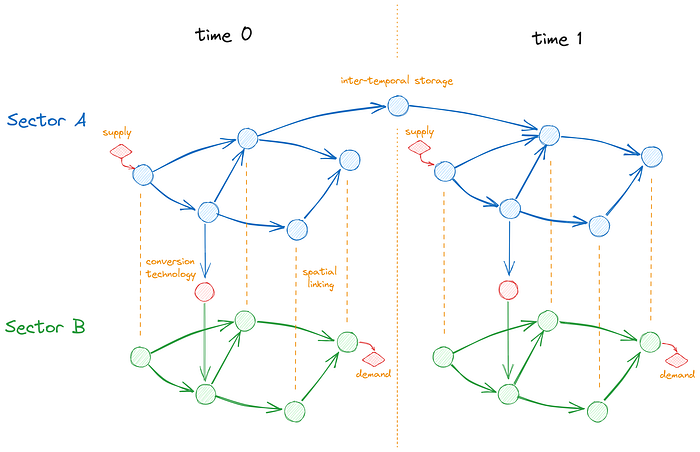
The overall problem is thus formulated by two simple continuity equations: first, demand for every commodity should be satisfied — at all nodes in the system, and at all time steps; and second, the net accumulation at each node of every commodity should be zero, i.e. supply and imports should equal demand and exports at each node. Many systems models also include a fixed, or ‘activation’ charge component, which can be used to represent an investment in supply capacity at a node, or transmission capacity across an edge. Constraints which are defined semantically in the model definition, such as constrained production, or limits to the growth of certain technologies through time, are also applied to the fixed and variable node and edge costs.
The constrained minimum-cost flow problem is NP-Hard.
Constraining to linear costs, the problem is able to be expressed as a mixed-integer linear programme, of the form:
minimize cᵀ x
subject to Ax ≤ b
and l ≤ x ≤ u
for decision variables x ∈ ℝⁿ, where c ∈ ℝⁿ is the coefficients of the cost function, A∈ ℝᵐˣⁿ are the coefficients of the constraints b ∈ ℝᵐ, and l ∈ ℝⁿ and u ∈ ℝⁿ are the lower and upper bounds of x respectively.
Optimisation of a linear system of equations uses a class of algorithms that are both exact (i.e. can demonstrate the optimality of their solution); and efficient. The solution algorithms do not massively benefit from parallelisation which means that; a) there is a practical limit to the size of a system that is represented; and b) organisations with extensive resources cannot buy or over-invest in their ability to design and solve systems models. An equalising effect, quality of the systems model is constrained by the available data, skill, and intuition of the systems modeller. Linear systems are also much more memory-efficient, which means that larger, high-fidelity systems can be described.
Linearity, however, has several consequences for the kind of economic logic that can be represented. Marginal costs for each producer are constant; scaling cost curves must be defined piece-wise with multiple constraints. Profitability cannot be represented or constrained directly, as prices (a function of quantities) and quantities themselves cannot be multiplied together. This can lead to model solutions which cannot be feasibly produced according to the model’s prevailing economic logic. For example, a least-costs energy investment model may recommend substantial investment in zero-marginal-cost renewable generating options, but these investments would reduce their own rents to zero, and the investments would not be profitable.
TransitionZero’s Future Energy Outlook
At TransitionZero, we’re building a systems modelling platform to help users jump directly in to their research questions. Our goal is to make systems modelling tools more accessible to beginners, and more useful to experts. Beginners will find our Future Energy Outlook platform comes with batteries-included: historic production data, technology parameter data, and default network configurations all available out-of-the-box, accessible via either a browser-based UI or an accessible Python client library. For experts, we provide rigorous analysis fast, allowing users to test their system boundaries, model fidelity, and input data sensitivities by rapidly scaling up ensembles of model runs.
Stay tuned for more progress updates about our Future Energy Outlook, and check out Part 2 for a hands-on tutorial where we start systems modelling from scratch!
